Trying Out Both Random Forest & Decision Tree Classifier On MNIST Using Scikit-Learn
It’s just a piece of cake. Let’s go!!
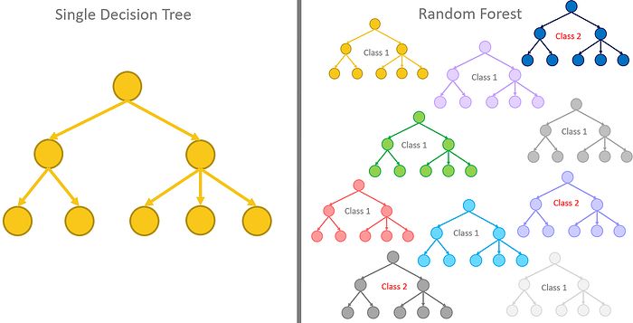
In the ‘Beginner’s guide to Random Forest Algorithm Classifier’ post, I explained why Random Forest is a much better algorithm to use when you have data with high dimensionality or a big data.
Today, I want to demonstrate how the two differ in terms of accuracy and robustness using the MNIST dataset which contains 60,000 greyscale images of handwritten digits.
Note : Though the MNIST dataset is quite large with 784 features, it is not regarded to be a high dimensionality dataset in most cases. Most High Dimensionality datasets have their number of features greater than or equal to the number of observations
I will train this dataset using a Decision Tree and a Random Forest so you can appreciate the strength and — of random forest.
First, we will import our needed modules from the scikit-learn library
from sklearn.ensemble import RandomForestClassifier
from sklearn.datasets import fetch_openml
from sklearn.model_selection import train_test_split
from sklearn.metrics import accuracy_score
from sklearn.tree import DecisionTreeClassifier
After importing our needed classes from the scikit library, we now load the MNIST dataset into the notebook
# loading the mnist dataset into the notebook
mnist = fetch_openml('mnist_784',version=1)
We split our dataset into training and test dataset. The X datasets are the features the model will learn from to predict the y’s.
More like how you look at a person’s physical features and guess with certainty who it could be without seeing their face. Because you have stored their features (gait, stature, head shape, etc ) in memory and can use it
# Split the dataset into training and test sets
X_train, X_test, y_train, y_test = train_test_split(mnist.data, mnist.target,
                                                    test_size=0.2,
                                                    random_state=42)
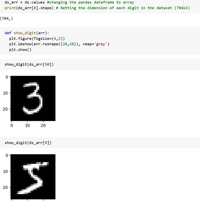
Digits From the MNIST Dataset
Training The Model Using A Random Forest
Now that we have our train and test datasets. We can instantiate the Random Forest Classifier for training the model to make the right predictions
# Instantiate a random forest classifier
rf = RandomForestClassifier(n_estimators=100, random_state=42)
# Fit the model to the training data
rf.fit(X_train, y_train)The ‘ fit ’ function instructs the model to learn the patterns in the data and adjust the parameters to minimize the error between the predicted and actual output. This process is called Training the Model. Here, the model is given both X_train and y_train to learn from, finding matching patterns in each observation or datapoint of the X_train that gives it corresponding y value.
It simply learns the patterns in the X that gives them their respective y values

The ‘predict’ function from the RandomForestClassifier class takes the X values of the test dataset then uses it to predict the corresponding y outputs. It learns from the X_test values using the pattern it learnt from the X_train dataset during training of the model.
Then uses the pattern from X_test to predict its output. The output should be same or near the values of the y_test. This is because X_test produces y_test and X_train produces y_train
Now let us calculate the accuracy of the model

The accuracy of the model using Random Forest Classifier is 96.7%
Training The Model Using A Decision Tree
# Instantiate a random forest classifier
dt = DecisionTreeClassifier(random_state=42)
Creating a decision tree model to compare with the accuracy of the Random Forest Algorithm
# Fit the model to the training data
dt.fit(X_train, y_train)
Using Decision Tree to train the model on the train dataset. The classifier model finds the patterns in X_train that makes it produce its corresponding y_train


The accuracy of the Decision Tree Model is 86.9%

Both models are trying to predict the values in y_test in the end with certainty. So let’s see which one was more accurate. From the accuracy of the two models, the Random Forest classifier should do a better job at predicting than the Decision Tree.
The RF scores an accuracy of 96.7% whiles the DT scores an accuracy of 86.7%. This clearly shows in their prediction, the first three values in the y_test(the values we are predicting) are [8, 4, 8,…]. The RF model predicted [8, 4, 8, … ] and the DT predicted [8, 4, 5, …]. Clearly showing the RF was more accurate.
For small datasets, RF and DT may have the same or almost the same accuracy.
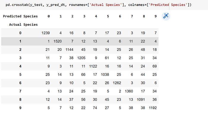
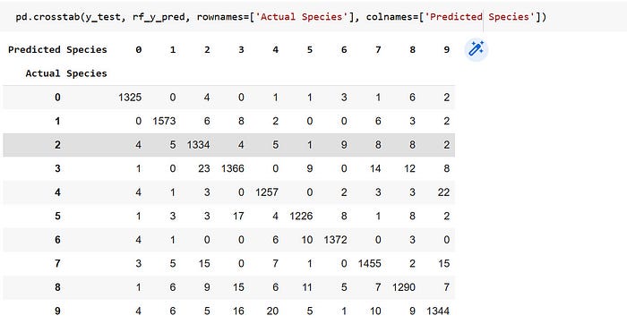
Confusion Matrix showing the Performance of Each Model
Breakdown of the Confusion Matrix of the Random Forest Algorithm
The rows of the matrix represent the true classes and the columns represent the predicted classes. The numbers in the matrix represent the counts of true positive (TP), false positive (FP), true negative (TN), and false negative (FN) classifications for each class.
- The first row represents the digit 0. The numbers in this row represent the number of times that the model correctly predicted digit 0 (TP = 1325), incorrectly predicted one of the other digits as digit 0 (FP = 0 + 4 + 1 + 4 + 1 + 4 + 3 + 1 + 4= 22), and incorrectly predicted digit 0 as one of the other digits (FN = 0 + 4 + 0 + 1 + 1 + 3 + 1 + 6 + 2= 18).
- The second row represents the digit 1. The numbers in this row represent the number of times that the model correctly predicted digit 1 (TP = 1573), incorrectly predicted one of the other digits as digit 1 (FP = 5 + 0 + 1 + 3 + 1 + 5 + 6 + 6 = 27), and incorrectly predicted digit 1 as one of the other digits (FN = 6 + 8 + 2 + 0 + 0 + 6 + 3 + 2= 27).
- The tenth row represents the digit 9. The numbers in this row represent the number of times that the model correctly predicted digit 9(TP = 1344), incorrectly predicted one of the other digits as digit 9(FP = 2 + 2+ 2+ 8 + 22 + 2 + 0 + 15 + 7= 60), and incorrectly predicted digit 9 as one of the other digits (FN = 4 + 6 + 5 + 16 + 20 + 5 + 1 + 10 + 9= 76).
Same applies to the confusion matrix of the Decision Tree.
NB: The true positives are always the diagonal figures in the matrix.
Yeah!! so that’s the end but not everything to it.
Where Do Data Scientist Go Camping?
A Random Forest!! Huh!!


